Listen, football injuries aren’t cool. I’ve elaborated on this in depth in my previous blog post so let me not bore you with further ramblings.
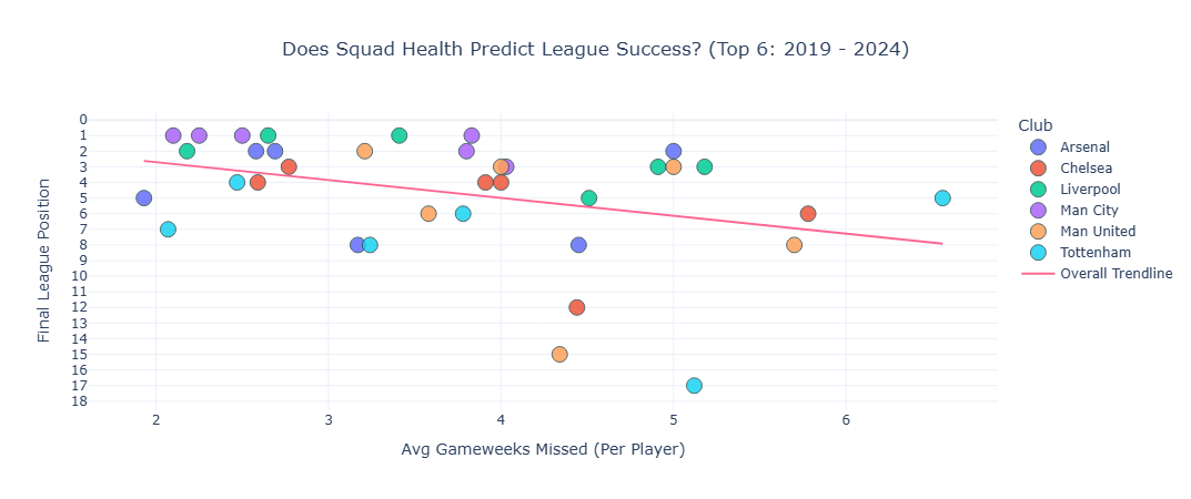
We know how critical injury prevention is for a Premier League team who want to win the league. The average number of gameweeks missed per player for a team closely correlates with that team’s final league position, and this is especially true for the top sides in England. The margins are extremely fine. The plot below shows us that teams who maintain lower average gameweeks missed per player are far more likely to finish in the top two. Or in other words, teams who top the average-gameweeks-missed-per-player board (with the lowest number) are most likely to also top the Premier League table!
This begs the question, how can a team prevent these injuries from happening? The answer may be found in survival analysis. Survival analysis models the time to an event and has the ability to convert this to a risk score over time. It helps the coaching staff and physio staff to know, at a given time, what is the injury risk score of player x.
The approach I took was to loosely follow the study by Catrell et al. (Catterall et al. 2026). Here a Survival Analysis was carried out on the SoccerMon dataset (Midoglu et al. 2022). SoccerMon is “A Large-Scale Multivariate Soccer Athlete Health, Performance, and Position Monitoring Dataset”. SoccerMon is the largest soccer athlete dataset available that tracks both subjective (using questionnaire methods) and objective features (using GPS trackers and other sensors). The data comes from two teams from the Norwegian women’s elite soccer league over the span of two years (2020-2021).
I used this paper to inform which features I extract from the SoccerMon dataset. Below is a list of the features I extracted. Each feature represents a 21 day moving average of that feature.
player_name |
Unique identifier/name of the player. |
|
date |
Date of the observation or training session. |
|
ATL |
Acute Training Load |
objective |
Weekly load |
Total accumulated training load over the last week. |
objective |
Monotony |
Training monotony metric |
objective |
Strain |
Training strain metric |
objective |
ACWR |
Acute:Chronic Workload Ratio |
objective |
CTL28 |
Chronic Training Load calculated over the previous 28 days. |
objective |
CTL42 |
Chronic Training Load calculated over the previous 42 days. |
objective |
Fatigue |
Self-reported fatigue score from the wellness questionnaire. |
subjective |
Mood |
Self-reported mood score from the wellness questionnaire. |
subjective |
Readiness |
Self-reported readiness-to-train score. |
subjective |
Sleep duration |
Number of hours slept prior to the report. |
subjective |
Soreness |
Self-reported muscle soreness score. |
subjective |
Stress |
Self-reported stress level score. |
subjective |
daily_load |
Total training load accumulated on that day. |
objective |
sRPE |
Session Rating of Perceived Exertion load, typically session duration × RPE. |
objective |
duration obj |
Objectively measured session duration. |
objective |
RPE |
Rating of Perceived Exertion reported by the athlete after the session. |
subjective |
Speed_km_h_mean |
Mean speed recorded during the session (km/h). |
objective |
Speed_km_h_max |
Maximum speed recorded during the session (km/h). |
objective |
Speed_km_h_std |
Standard deviation of speed during the session. |
objective |
Distance |
Total distance covered during the session. |
objective |
distance_per_min |
Average distance covered per minute of activity. |
objective |
total_time_min |
Total duration of the session in minutes. |
objective |
sp_lir_t |
Time spent in the Low-Intensity Running speed zone. |
objective |
sp_lir_d |
Distance covered in the Low-Intensity Running speed zone. |
objective |
sp_lir_p |
Percentage of total session spent in the Low-Intensity Running speed zone. |
objective |
sp_mir_t |
Time spent in the Moderate-Intensity Running speed zone. |
objective |
sp_mir_d |
Distance covered in the Moderate-Intensity Running speed zone. |
objective |
sp_mir_p |
Percentage of total session spent in the Moderate-Intensity Running speed zone. |
objective |
sp_hir_t |
Time spent in the High-Intensity Running speed zone. |
objective |
sp_hir_d |
Distance covered in the High-Intensity Running speed zone. |
objective |
sp_hir_p |
Percentage of total session spent in the High-Intensity Running speed zone. |
objective |
sp_spr_t |
Time spent sprinting. |
objective |
sp_spr_d |
Distance covered while sprinting. |
objective |
sp_spr_p |
Percentage of total session spent sprinting. |
objective |
has_gps_data |
Indicator that GPS measurements are available for the session. |
objective |
has_session_data |
Indicator that session/training load data are available. |
objective |
wellness_reported |
Indicator that the athlete completed the wellness questionnaire. |
objective |
is_rest_day |
Indicator that the day was designated as a rest day. |
objective |
is_injured_today |
Indicator that the player was injured on the given date. |
objective |
injury_onset |
Indicator marking the first day of an injury event. |
objective |
event |
Survival-analysis event indicator |
objective |
time_to_event |
Survival-analysis time-to-event variable (days) |
derived |
Extensive EDA and necessary transformations (StandardScaler for columns with a normal distribution and Yeo-Johnson scaling for skewed data) were applied. These transformations help the model see the patterns in the data better as it places all the numbers on the same scale. Without transformations any column with large numbers like Speed_km_h_mean compared to columns with smaller numbers like ACWR will dominate the model during training.
Two further features were added to the dataset, and that was event and time-to-event. Where event is a boolean value (0 or 1) denoting if a player got injured within the next seven days (1) or not (0). Time-to-event was the number of days leading up to the event (starting at 7 days back). See an example of the unscaled dataset below:
| 1143 |
TeamB-29c5271b-5c46-455e-91ea-da2abfa8ff3c |
2020-08-10 |
0 |
0 |
0 |
7 |
233.673333 |
1635.714286 |
1.699048 |
2900.757143 |
... |
0.060317 |
0.021745 |
0.000379 |
0.000317 |
0.000133 |
0.000001 |
0.285714 |
0.857143 |
0.809524 |
0.142857 |
| 1144 |
TeamB-29c5271b-5c46-455e-91ea-da2abfa8ff3c |
2020-08-11 |
0 |
0 |
0 |
7 |
239.047619 |
1673.333333 |
1.743333 |
2987.342857 |
... |
0.071905 |
0.026021 |
0.000443 |
0.001429 |
0.000605 |
0.000007 |
0.333333 |
0.857143 |
0.809524 |
0.142857 |
| 1145 |
TeamB-29c5271b-5c46-455e-91ea-da2abfa8ff3c |
2020-08-12 |
0 |
0 |
0 |
7 |
243.197619 |
1702.380952 |
1.778095 |
3060.814286 |
... |
0.139524 |
0.050366 |
0.001400 |
0.006984 |
0.003020 |
0.000086 |
0.380952 |
0.809524 |
0.809524 |
0.190476 |
| 1146 |
TeamB-29c5271b-5c46-455e-91ea-da2abfa8ff3c |
2020-08-13 |
0 |
0 |
0 |
7 |
244.490476 |
1711.428571 |
1.800000 |
3100.466667 |
... |
0.139524 |
0.050366 |
0.001400 |
0.006984 |
0.003020 |
0.000086 |
0.380952 |
0.809524 |
0.809524 |
0.190476 |
| 1147 |
TeamB-29c5271b-5c46-455e-91ea-da2abfa8ff3c |
2020-08-14 |
0 |
0 |
0 |
7 |
243.878571 |
1707.142857 |
1.803810 |
3099.347619 |
... |
0.182540 |
0.066014 |
0.001636 |
0.007619 |
0.003287 |
0.000090 |
0.428571 |
0.809524 |
0.809524 |
0.190476 |
5 rows × 45 columns
So, how do we use these features to inform us whether a player is at a high risk of injury or not? Well, this is where Survival Analysis comes into play. For this problem I have used the Random Forest Survival model and trained it on the features we see above using a leave one player out process. This means the model was trained on every player except one and then the trained model was applied to that one player to mimic a real world application. This process was repeated with each player.
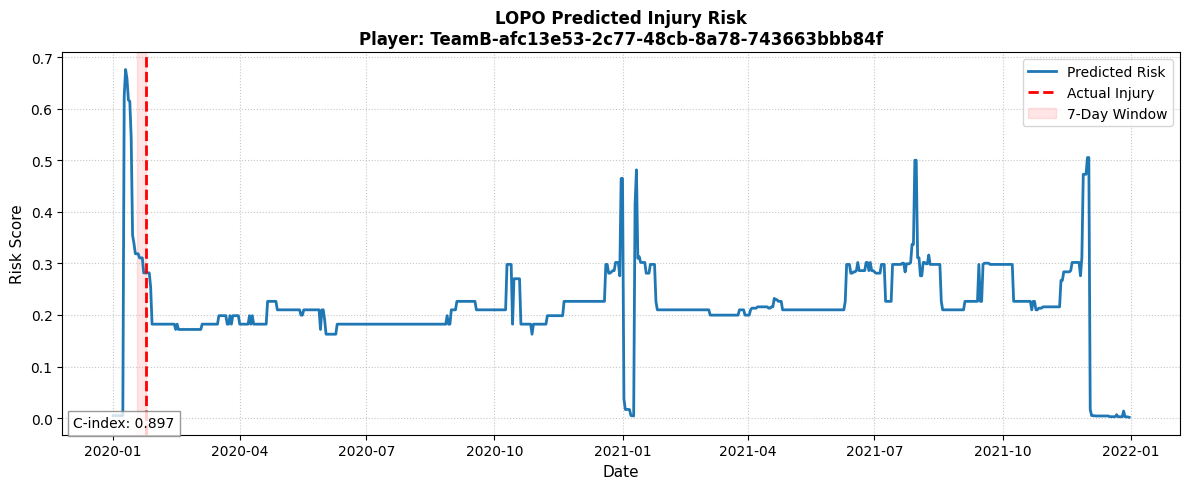
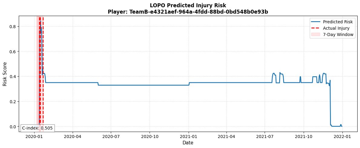
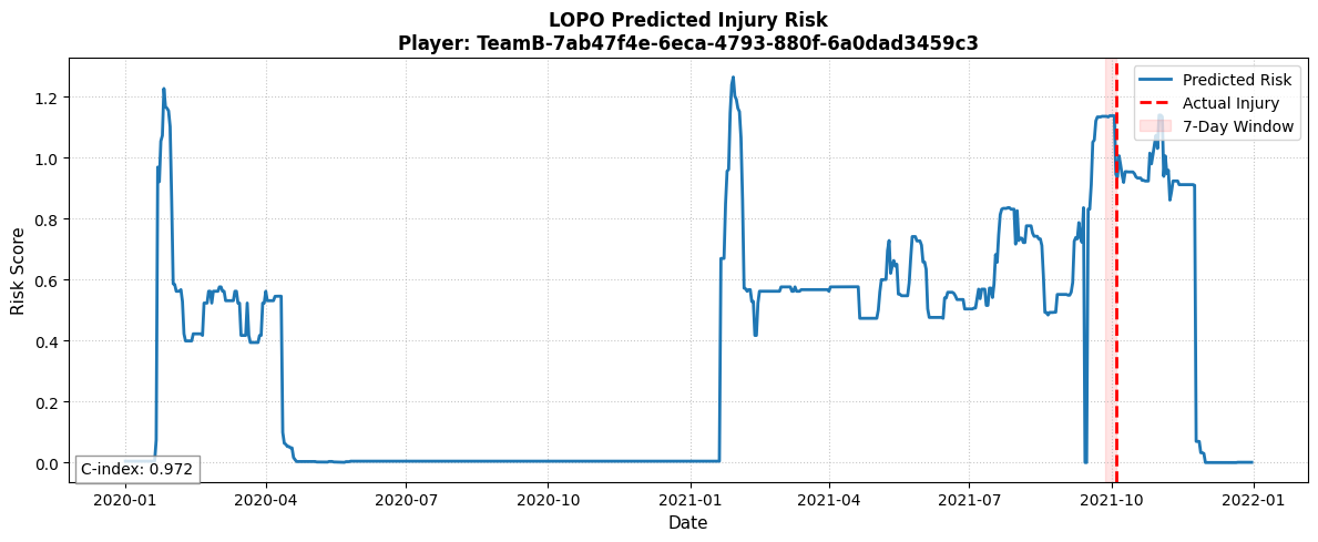
The results are promising! The plots below show player injury risk over time with a vertical line showing where an injury actually occured. Notice how the injuries always occur around where an increased injury risk is!
These plots visualise how the risk value corresponds with actual injury periods. Before each injury there is a peak in injury risk. This can serve as an incredibly valuable tool in managing player load and injury prevention. One may note that there are periods of heightened injury risk where no injury ultimately occurs. This is simply the nature of the sport. A player may be teetering on the edge, but through a combination of luck and good, intuitive management by the coaching staff, they avoid injury and remain available for those all-important gameweek fixtures.
Notice the C-index score at the bottom left of each plot. The c-index means essentially how well the model ranks danger rather than predicting exact futures. Because sports injuries are relatively rare, the model could theoretically be 99% “accurate” simply by guessing that no one ever gets hurt (which is completely useless to a coaching staff).
Instead, the C-index grades the model like an Emergency Room triage nurse. Just as a triage nurse doesn’t predict exactly when a patient will heal but correctly prioritizes someone with chest pains over someone with a paper cut, the C-index evaluates prioritisation. It looks at a player’s timeline and asks: If we randomly pick one healthy training day and one actual pre-injury day, did the model correctly assign a higher risk score to the dangerous day? A score of 0.50 means the model is effectively flipping a coin, 0.70 indicates a solid ranking ability, and anything over 0.80 means you have a highly reliable early-warning system to keep your squad on the pitch.
These risk scores are great at finding portions in the season where a player may get injured, but what does the coach or physio do about this? It will be very difficult to tell the coach to go easy on a player just because a blue line is high and not low. And then again, what does “go easy on a player” even mean? Does that mean don’t play them in the next match, give them a day off, just give them light drills, etc?
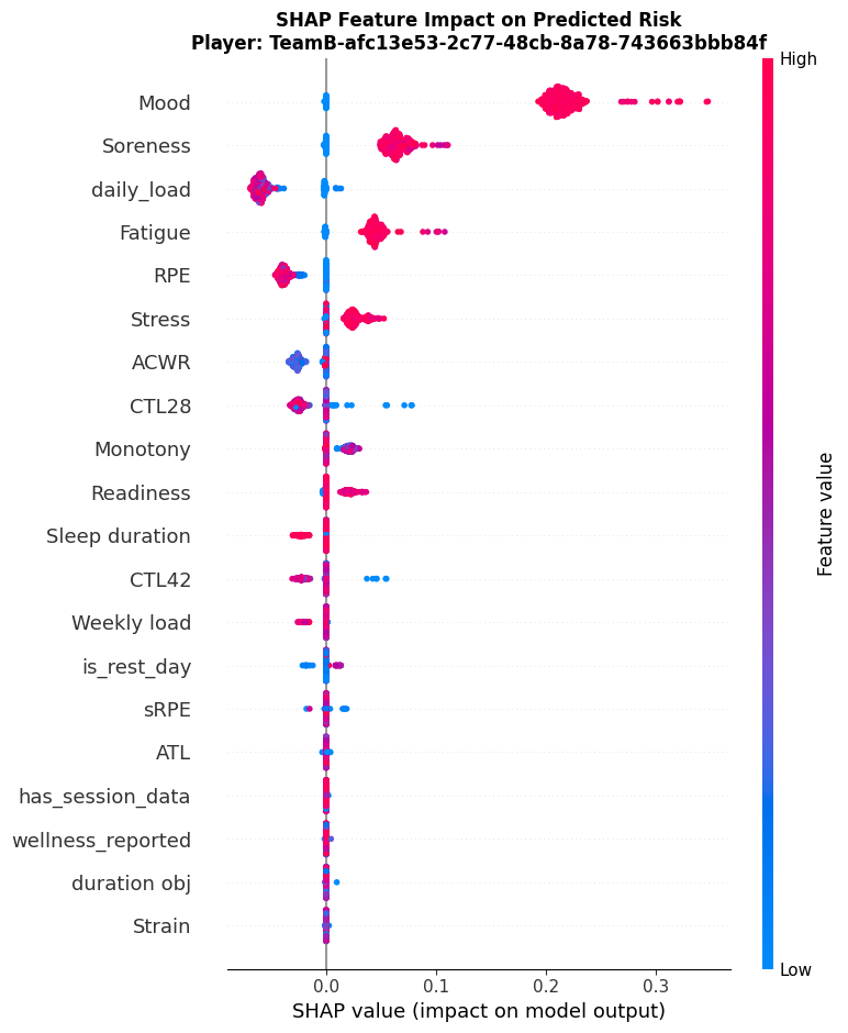
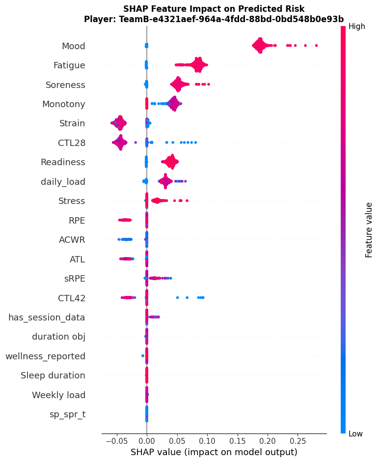
SHAP analysis can answer these questions, not just on a global level but at a player specific level! Take a look at the SHAP values below for Player A and Player B.
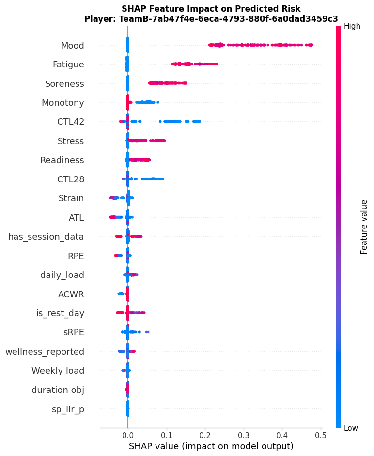
These plots are known as beeswarm plots. Each dot represents a feature’s scores for a specific day, the colour of that dot represents whether the score for that feature was high (red) or low (blue) and the position of the dot tells us if the feature value pushed the model to predict a higher risk of injury (right) or lower risk of injury (left)
Let’s zoom in on what we are seeing for Player A:
- Mood, soreness, daily_load, fatigue, RPE, stress influence the risk score the most.
- Higher than normal mood scores are pushing the injury risk upwards!?
- Higher than normal levels of soreness are pushing the injury risk upwards
- A bit of a mix for daily_load but higher levels seemed to stand out and could perhaps be beneficial for Player A
- Higher than normal levels of fatigue push the injury risk upwards
- Higher than normal ratings of RPE (Rating of Perceived Exertion) decrease the injury risk for Player A
- Higher than normal stress levels increase the risk of injury for Player A.
Now let’s zoom in on Player B:
- Player B shows the same pattern for mood, fatigue and soreness
- Higher than normal readiness scores push the injury risk upwards for Player B
- Higher than normal levels of strain reduces the injury risk for Player B
- Higher than normal levels of CTL28 reduces the injury risk for Player B
Player C seems to follow a similar pattern portrayed for Player A and B with regards to mood, fatigue and soreness.
Conclusion
Survival analysis is a great tool to mitigate player injuries for a sports team with a Random Forest Survival model being one of the highest performing models for this task. While injury risk overtime is great, understanding what drives that risk up or down is equally as important.
Features that drive risk scores are not always intuitive and differ from player to player. For one player higher intensity training may actually reduce injury risk. Some intuitive features show that increased levels of perceived soreness and fatigue lead to injury risk. More unintuitive outcomes show that higher than normal mood scores actually increase risk injury. Given that mood score is a very subjective metric it is difficult to say what one player means to be a “good” mood compared to another.
Overall, there is considerable promise in combining Survival Analysis with SHAP-based interpretability at the individual player level to quantify and understand injury risk over time.
References
Catterall, Victoria, Cise Midoglu, and Stephen Lynch. 2026.
Time-to-Injury Forecasting in Elite Female Football: A DeepHit Survival Approach.
https://arxiv.org/abs/2601.19479.
Midoglu, Cise, Matthias Boeker, Andreas Kjæreng Winther, et al. 2022.
“SoccerMon: A Large-Scale Multivariate Soccer Athlete Health, Performance, and Position Monitoring Dataset.” Version v1. Zenodo.
https://doi.org/10.5281/zenodo.10033832.